Back to undergraduate research page
Fractional Gompertz models
This work led to a joint publication with a student here!

The Gompertz dynamic equation (investigated here) is $$y^{\Delta} = (\ominus r)yL_y(t,t_0),$$ where $L_y$ denotes the Bohner logarithm. In the case of the time scale $\mathbb{T}=\{0,1,2,\ldots\}$, the Gompertz dynamic equation becomes the difference equation $$\Delta y = \left(-\dfrac{r}{1+r}\right)yL_y(t,t_0), \quad L_y(t,t_0)=\displaystyle\sum_{k=t_0}^{t-1} \dfrac{y(k+1)-y(k)}{y(k)}.$$ An analogous $\nabla$ equation can be defined as $$\nabla y = \left(\boxminus r\right)yL_y(t,t_0), \quad L_y(t,t_0)=\displaystyle\sum_{k=t_0+1}^t \dfrac{y(k)-y(k-1)}{y(k)}.$$ In this article published with an undergraduate, we defined three discrete fractional logarithms: $$L_{y,\nu}(t,t_0)=\left( \nabla_{t_0}^{-\nu} \dfrac{y^{\nabla}}{y}\right)(t), \quad t\in\mathbb{N}_{t_0+1},$$ $$\ell_{y,\nu}(t,t_0)=\displaystyle\int_{t_0}^t \dfrac{\nabla_{t_0}^{\nu} y(\tau)}{y(\tau)} \nabla \tau, \quad t \in \mathbb{N}_{t_0+1},$$ and $$\Lambda_{y,\nu}(t,t_0)=\left( \nabla_{t_0}^{-\nu}\dfrac{\nabla_{t_0}^{\nu} y}{y} \right)(t), \quad t \in \mathbb{N}_{t_0+1}.$$ With these three logarithms, we studied three Riemann-Liouville fractional difference initial value problems: $$\nabla y = (\boxminus r)y(a+L_{y,\nu}), \quad y(t_0)=y_0, \hspace{35pt} (*)$$ $$\nabla_{t_0}^{\nu} y(t) = (\boxminus r)y(a+\ell_{y,\nu}), \quad y(t_0+1)=y_0,$$ and $$\nabla_{t_0}^{\nu} y(t)=(\boxminus r)y(a+\Lambda_{y,\nu}), \quad y(t_0+1)=y_0.$$ We found a closed form solution of $(*)$ in terms of the (Riemann-Liouville) discrete Mittag-Leffler function as follows: if $0<\nu<1$, $r<\dfrac{1}{2}$ and for $t \in \mathbb{N}_0$, and $\displaystyle\sum_{k=t_0+1}^t E_{\boxminus r,\nu,\nu-1}(t-k+1+t_0,t_0)H_{-\nu}(k,t_0) \neq -1 - \dfrac{1-r}{ar}$, then (*) has the unique solution $y(t)=y_0 E_p(t,t_0)$, where $p(t)=(\boxminus r)a+(\boxminus r)\Big( E_{\boxminus r,\nu,\nu-1}(\cdot,t_0) * aH_{-\nu}(\cdot,t_0)\Big)(t)$. Closed-form solutions of a wider range of parameters or the other two models were not achieved.

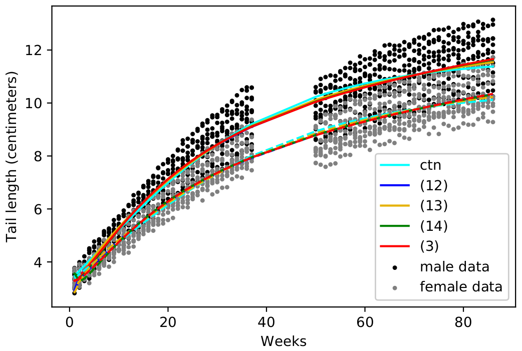
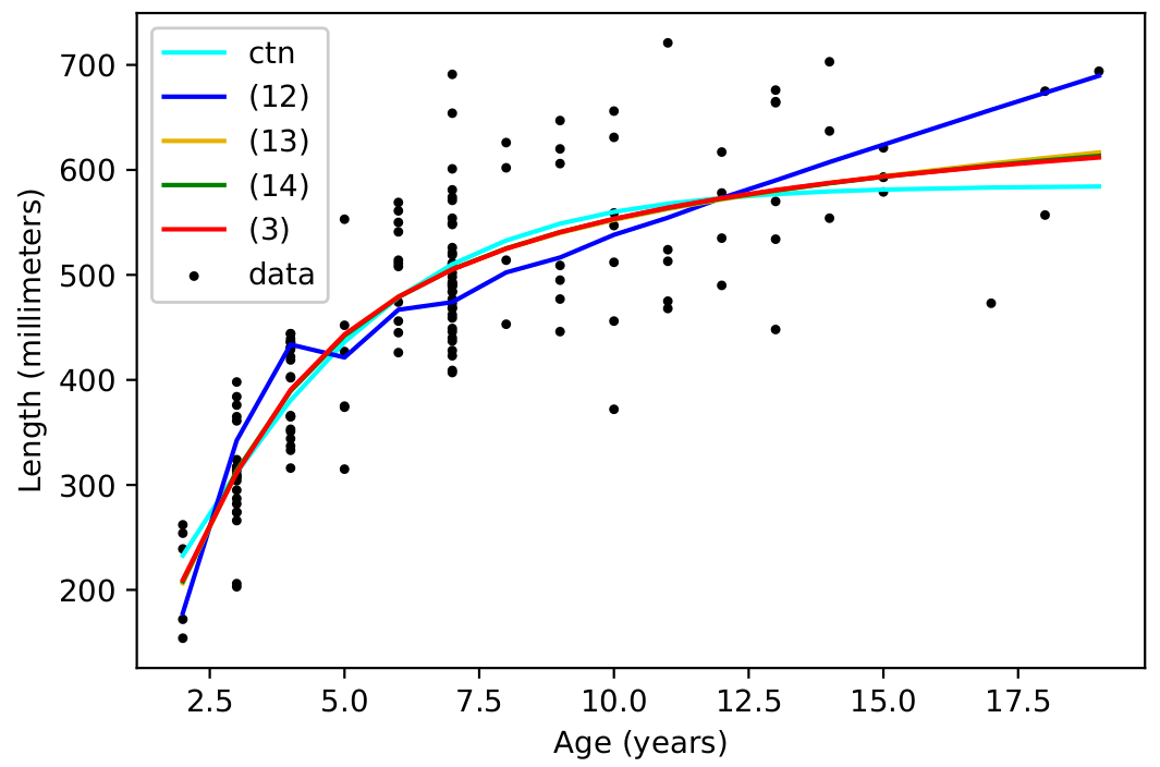
The three models were fit to data and compared to pre-existing models. It was shown that they fit some data equally well to the pre-existing models (including the long-existing continuous model for $\mathbb{T}=\mathbb{R}$). The first image is data collected measuring tail length of male and females of a species of skinks; the second image is fit to data comparing the age to the length of certain catfish caught in Cheat Lake, West Virginia:
Python source code for solutions to these equations can be found here.

Some potential projects for further research

1. Change the time scale from $\mathbb{T}=\{0,1,2,\ldots\}$ to another time scale. This will cause the coefficient $\ominus r$ to be a function of time instead of being a constant.
2. Investigate qualitative properties of the existing discrete models. For instance, characterizing when solutions are stable or oscillatory.
3. Repeat the analysis in the discrete case for other fractional differences such as the Caputo difference.